Machine Learning 101 with Microsoft ML.NET (part 2/3)

The purpose of this series of articles is to provide a complete guide (from data to predictions) to machine learning, for .NET developers in a .NET ecosystem, that is now possible using Microsoft ML.NET and Jupyter Notebooks. Even more, you don’t have to be a data scientist to do machine learning.

4. Model builder pipeline

At the end of the first part of this series, we had a preprocessing pipeline ready to load data and concentrate the features selected for the training into one special feature called Features, and a target feature named Label serving as a category where the selected features classifies. If we don’t have such a column as Label in our dataset, we have to annotate the target field it follows (of course, for another problem, we may have another target feature we need to annotate):

[ColumnName("Label")]
public string Source { get; set; }

Dimensionality Reduction

Our intuition tells us, from the machine learning model prediction perspective, that we need as many features as possible. But from the performance perspective we need as little as we can to solve our problem. Indeed, sometimes a faster machine learning model is preferable to a more performant one. The correlation matrix is just one way to decide which features to keep for classification and regression models. Another way is the PFI (Permutation Feature Importance).

ML Context

Before proceeding to build the training pipeline, let me introduce the MLContext catalog container. Inside this object, we can find all the trainers, data loaders, data transformers, and predictors used for a large set of tasks like: regression, classification, … Many of them are part of additional nuget packages to keep the main libraries more lightweight. The seed parameter is useful (e. g. for unit tests) if you want to have a deterministic behavior, since this is used by splitters and some trainers.

What is an ML trainer?

There are multiple training algorithms for every kind of ML.NET task available as trainers which can be found in their corresponding trainer catalogs. For example, Stochastic Dual Coordinated Ascent which we used in this article is available as Sdca (for regression), SdcaNonCalibrated and SdcaLogisticRegression (for binary classification), and SdcaNonCalibrated and SdcaMaximumEntropy (for multi-classification).

Let’s go back to the preprocessing pipeline created in the first part of this article:

var featureColumns = new string[] { "Temperature", "Luminosity", "Infrared", "Distance" };
var preprocessingPipeline = mlContext.Transforms.Conversion.MapValueToKey("Label")
  .Append(mlContext.Transforms.Concatenate("Features", featureColumns));

We can now continue by extending the pipeline and selecting a trainer.

var trainingPipeline = preprocessingPipeline.Append(mlContext.MulticlassClassification.Trainers.SdcaNonCalibrated("Label", "Features"));

We are not done until we do the post-processing, which in our case is simply mapping the key to value in order to make the prediction human-readable (see above the mapping from value to key in the preprocessing pipeline).

var postprocessingPipeline = trainingPipeline.Append(mlContext.Transforms.Conversion.MapKeyToValue("PredictedLabel"));

Is the training pipeline enough to create the model? Of course not, we need to feed in some data in order to get the model trained. Please notice that until we call the Fit method on our pipeline, we don’t get any piece of data from the loader except its schema, and that’s because the DataView is lazy-loading (you can think of it as a Linq IEnumerable).

var model = postprocessingPipeline.Fit(trainingData);

Weights and biases

At its very core, a trainer is a generic algorithm which has the ability to tune its weights and biases by training on data. The more data, the better the tuning.

VBuffer[] weights = default;
model.Model.GetWeights(ref weights, out int numClasses);
var biases = model.Model.GetBiases();

5. Model Builder and Automated ML

Perhaps the first concern of a developer when it comes to machine learning is choosing a good trainer, but this should not be an exclusively data scientist task. ML.NET includes an excellent technology called Automated ML (AutoML), which comes in different flavors such as:

• Visual Studio UI tool (An integrated wizard called Model Builder for generating ready-to-use code)
• ML.NET CLI tool (You can install it as a global tool, and once installed, you can give it a machine learning task and a training dataset. It generates an ML.NET model, as well as the C# code to run to use the model in your application.)

mlnet regression --dataset "sensors_data.csv" --train-time 600

• Code (You can integrate it into your code)

var experimentResult = Context.Auto()
  .CreateMulticlassClassificationExperiment(ExperimentTime)
  .Execute(trainingDataView);
var bestRun = experimentResult.BestRun;
var model = bestRun.Model;

6. Measuring the model quality

Validate the model

I have already mentioned the model performance a few times already, but how can we measure that? A well-known validation technique is cross-validation (fig. 1 and 2), which can be used to tune the hyperparameters. A hyperparameter is a parameter used to control the learning process. We can find and modify it in the method signature of a trainer. Model parameters are internal to models and can be learned directly from the training data, but hyperparameters cannot.

var crossValidationResults = mlContext.MulticlassClassification.CrossValidate(trainingData, postprocessingPipeline, numberOfFolds: 5, labelColumnName: "Label");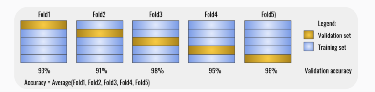

The cross-validation is checking for model consistency. It is basically:

1. Divides the dataset into k sub-datasets (folds)
2. Trains the model on k – 1 folds and leaves one fold for testing
3. Evaluates the model on testing fold
4. Repeats the previous steps for another set of k – 1 folds so the testing fold is different than previous testing folds used before
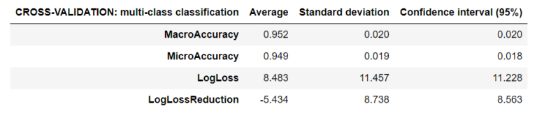
5. Computes the average metrics, standard deviation, and confidence interval

Please notice that cross-validation is pretty time-consuming since it’s training the model k times. We should not care too much since it is not done in production. More importantly is that it’s a good choice when only a limited amount of data is available, because the cross-validation is re-using the data from the training dataset.

PFI (Permutation feature importance)

By randomly shuffling the dataset data one feature at a time we measure the importance of a feature by calculating the increase in the model’s prediction error after permuting the feature. A larger change indicates a more important feature, so we can select the most important features (focusing on using a subset of more meaningful features) to build our model. In this way we can potentially reduce noise and training time.

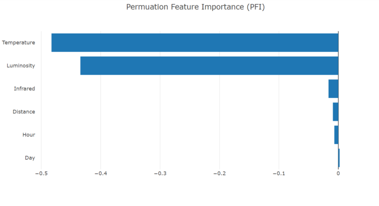
Adding a strongly correlated feature is expected to decrease the importance of the associated feature. In figure 3 we can see the features Day and Hour, and maybe even Distance, can be removed without notable impact on the model performance.

var transformedData = model.Transform(trainingData);
var linearPredictor = model.LastTransformer;
var permutationMetrics = mlContext.MulticlassClassification.PermutationFeatureImportance(linearPredictor, transformedData);

Evaluate the model

Evaluation has similar metrics to validation, but they are very different in terms of scope. The evaluation is done on the testing dataset, which was put aside when we split the original dataset and didn’t take part in the training process at all (fig. 4).

var predictions = model.Transform(testingData);
var metrics = mlContext.MulticlassClassification.Evaluate(predictions, "Label", "Score", "PredictedLabel");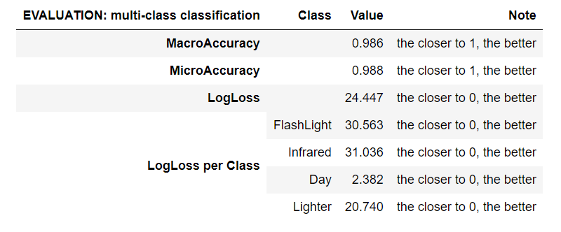

Normalization

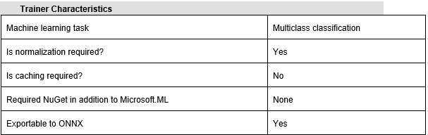
The first impulse is to consider the impact (or the weight, if you like) of each of the features on the model being the same. No matter their type (texts, categories, singles, doubles) for machine learning they are all numbers and, obviously, 0.1 or 100 will have different impacts, therefore they have to be normalized. If we miss normalizing our features, we risk training a bad model.

Some trainers don’t require explicit normalization (they are normalizing the features implicitly), but other trainers do. Fortunately, we don’t have to know the algorithm in order to decide that, because we can find the description of a trainer in the official documentation.

var preprocessingPipeline = mlContext.Transforms.Conversion.MapValueToKey("Label")
  .Append(mlContext.Transforms.CustomMapping<CustomInputRow, CustomOutputRow>
    (CustomMappings.IncomeMapping, nameof(CustomMappings.IncomeMapping)))
  .Append(mlContext.Transforms.Concatenate("Features", featureColumns))
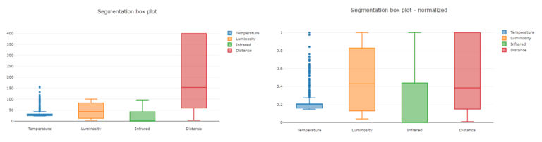
  .Append(mlContext.Transforms.NormalizeMinMax("Features"));

Let’s take a look over the box plot diagrams before and after normalization and compare the Distance to Temperature (fig. 5). The Distance will have a bigger impact on the model before normalization.

Evaluation Metrics

Micro-Accuracy aggregates the contributions of all classes to compute the average metric. The closer to 1.00, the better. In a multi-class classification task, micro-accuracy is preferable over macro-accuracy if you suspect there might be class imbalance.

Macro-Accuracy is the average accuracy at the class level. The accuracy for each class is computed and the macro-accuracy is the average of these accuracies. The closer to 1.00, the better.

Log-Loss measures the performance of a classification model where the prediction input is a probability value between 0.00 and 1.00. The closer to 0.00, the better. The goal of our machine learning models is to minimize this value.

Log-Loss reduction can be interpreted as the advantage of the classifier over a random prediction. Ranges from -inf and 1.00, where 1.00 is perfect predictions and 0.00 indicates mean predictions. For example, if the value equals 0.20, it can be interpreted as “the probability of a correct prediction is 20 % better than random guessing”.

Confusion Matrix

Along with micro-accuracy, macro-accuracy and log-loss, we can measure the confusion matrix. Using the testing dataset we can make predictions and compare the predicted results to the actual results and we can arrange them in a confusion matrix (fig. 6).

var metrics = mlContext.MulticlassClassification.Evaluate(predictions, Label, Score, PredictedLabel);
Console.WriteLine(metrics.ConfusionMatrix.GetFormattedConfusionTable());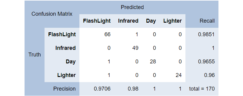

In the previous diagram we can see the FlashLight class was predicted correctly (as FlashLight source) 66 times, incorrectly as Day one time, and Lighter one time as well, resulting in a 0.9706 precision rate.

7. Save the model

After experimenting with different sets of features, trainers, and parameters building a machine learning model, we choose one which best fits to our needs. Most likely we need the model in a production scenario, so we have to persist the model to a physical file in native (ML.NET) format or in ONNX format (which is a portable format developed by Microsoft and Facebook and adopted by other big players too). Unsurprisingly, if you take a look at the file (for the native format), you will realize it’s a zip of text files containing numbers.

Saving the model in native format:

mlContext.Model.Save(model, trainingData.Schema, MODEL_PATH);

Saving the model in ONNX format:

using (var stream = System.IO.File.Create(ONNX_MODEL_PATH))
mlContext.Model.ConvertToOnnx(model, trainingData, stream);

Load the native model:

var trainedModel = mlContext.Model.Load("model.zip", var out modelSchema);

part 3/3